Table of Contents
ToggleIntroduction
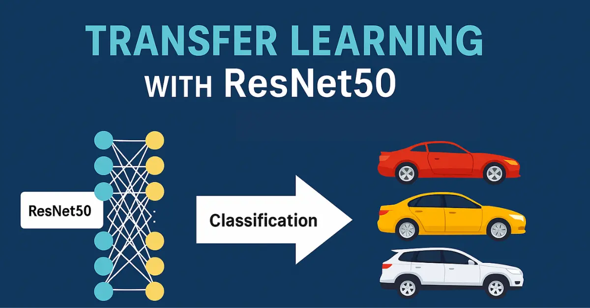
Transfer learning is a powerful technique that lets us take advantage of models already trained on massive datasets and adapt them to our own use cases. For example, researchers collected millions of images in a dataset called ImageNet and trained a deep model called ResNet50. This model learned to recognize general image features like edges, corners, textures, and shapes. Its main job is to classify images into 1,000 categories, such as apple, car, monitor, or pencil.
But here’s the catch: if we ask this model a very specific question, like “Is this a 2000 Hummer SUV or a 2010 BMW sedan?”, it struggles. It wasn’t trained to distinguish cars at that fine level.
This is where transfer learning comes in. Instead of training a huge model from scratch (which would take enormous time, data, and compute), we keep most of ResNet50’s “knowledge” and only retrain the last part of the network, the classification head, on our new dataset. In this project, that dataset is the Stanford Cars dataset, which contains 196 different car models.
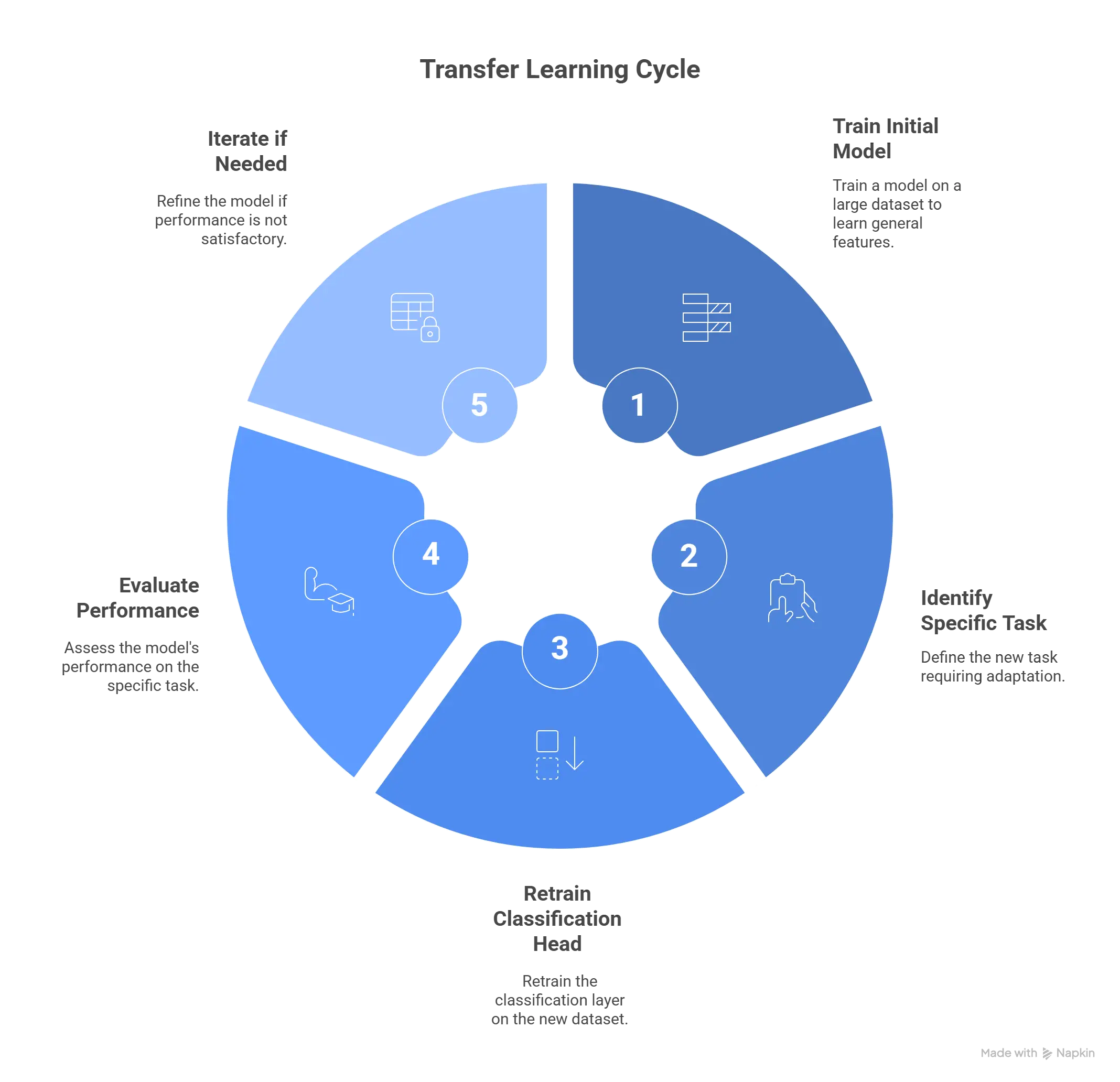
Think of it like a student who already knows how to read and write. If you hand them a car manual, they don’t need to relearn the alphabet, they just need to learn the specific terms and details about cars. In the same way, ResNet50 doesn’t need to relearn edges and corners; it only needs to adjust to car-specific features.
And if retraining just the last layers isn’t enough, we can go further and retrain some of the earlier layers too. That’s called fine-tuning, and it gives the model even more ability to adapt to our dataset. Of course, all this training requires significant compute power, which is why using a GPU is highly recommended (see my earlier post on GPU Acceleration with WSL2).
By the end, you will:
- Leverage a pre-trained ResNet50 model and adapt it to your own business or research needs.
- Apply this approach to specialized datasets, as we demonstrate with the Stanford Cars dataset, to refine the model for fine-grained tasks like classifying specific car models.
- Understand how data preprocessing, augmentation, and transfer learning work together to reduce training time and improve accuracy.
- Evaluate model performance through metrics, learning curves, and error analysis to guide further improvements.
- Recognize when to rely on transfer learning alone and when to extend it with fine-tuning for even greater accuracy.
Stanford Cars Dataset
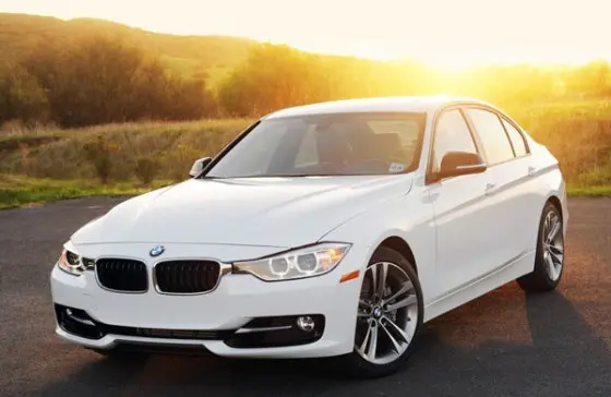
The Stanford Cars dataset is a benchmark for fine-grained image classification. It contains over 16,000 images across 196 different car models, ranging from sedans to SUVs to sports cars. Each image is labeled with its make, model, and year, which makes it an ideal dataset for testing how well transfer learning can handle subtle differences.
Dataset Statistics
The Stanford Cars dataset is relatively small compared to ImageNet but still large enough to train and evaluate deep models. Its structure makes it ideal for testing transfer learning.
Total images: 16,185
Training set: 8,144 images
Testing set: 8,041 images
Number of classes: 196
Images per class: Around 80 on average (fairly balanced)
Each class corresponds to a specific car make, model, and year. For example, “2008 Honda Accord Sedan” and “2009 Honda Accord Sedan” are treated as separate classes.
👉 This level of detail makes the dataset a strong benchmark for fine-grained classification, where models must learn to recognize subtle differences between categories.
Dataset Structure
To train effectively, images should be organized into a standard directory structure:
/cars/
    train/
        Acura Integra Type R 2001/
            img001.jpg
            img002.jpg
            ...
        Audi TT Hatchback 2011/
            img101.jpg
            ...
        ...
    validation/
        Acura Integra Type R 2001/
        Audi TT Hatchback 2011/
        ...
    test/
        Acura Integra Type R 2001/
        Audi TT Hatchback 2011/
        ...
- Each class (car model) has its own folder.
- Training, validation, and test sets all contain images, organized by class name.
- This structure allows
ImageDataGenerator.flow_from_directoryto automatically map folders to labels.
👉 With the dataset prepared and organized, the next step is to apply data preprocessing and augmentation before feeding images into the ResNet50 model.
Challenges in the Dataset
- Cars look very similar
Small changes between models or years make it hard for the model to notice the difference. - Same brand, many alike designs
For example, different BMW sedans may look almost the same, so the model can confuse them. - Different photo styles
Some images are in bright light, some in shadows, some in busy streets. This makes learning harder. - Few images per class
With only about 80 pictures for each car type, the model can easily memorize instead of learning.
👉 These issues explain why the dataset is challenging and why transfer learning is needed.
Data Preprocessing and Augmentation
Before ResNet50 can learn from our car images, we need to make sure the data is prepared properly. There are two things happening here:
Preprocessing: ResNet50 was originally trained on ImageNet, and it expects inputs in the same format. So we run every image through the
preprocess_inputfunction to scale the pixels exactly the way the backbone model expects.Augmentation: Our dataset isn’t huge (around 80 images per class), so the model could easily just memorize them. To make training more realistic, we apply random transformations; flipping, rotating, shifting, so each epoch the model sees slightly different versions of the cars.
Step 1: Set image size and batch size
All images are resized to 224 × 224 pixels, which is what ResNet50 takes as input. The batch size is 32, which is a safe number for our 4 GB GPU (My personal Laptop). We also fix a random seed so results are reproducible.
IMG_SIZE = (224, 224)   # resize everything to ResNet50’s default
BATCH_SIZE = 32         # how many images per step
SEED = 42               # keep runs reproducible
Step 2: Define the training generator
Here’s where the magic happens. We load images from the training folder and apply random transformations:
- Flip horizontally → cars can appear from left or right.
- Rotate slightly (±8°) → simulates tilted camera angles.
- Shift up/down/left/right → like framing differences in photos.
- Zoom in/out (±10%) → different levels of cropping.
- Shear → makes the image look slanted, as if shot from a corner.
- Brightness changes (85%–115%) → day vs evening lighting.
- Channel shift → tiny changes in colors.
- Fill with reflection → if shifting leaves empty pixels, fill them by mirroring the image.
from tensorflow.keras.preprocessing.image import ImageDataGenerator
from tensorflow.keras.applications.resnet50 import preprocess_input

train_datagen = ImageDataGenerator(
    preprocessing_function=preprocess_input,
    horizontal_flip=True,
    rotation_range=8,
    width_shift_range=0.1,
    height_shift_range=0.1,
    zoom_range=(0.9, 1.1),
    shear_range=0.1,
    brightness_range=(0.85, 1.15),
    channel_shift_range=10.0,
    fill_mode='reflect'
)
Step 3: Validation and test generators
For validation and test sets, we don’t add random changes, we only preprocess the images. This way, we measure performance on the real data, not on augmented versions.
val_test_datagen = ImageDataGenerator(
    preprocessing_function=preprocess_input
)
Step 4: Create generators for each split
Finally, we point each generator to the correct directory. Keras takes care of assigning labels based on folder names.
# NOTE: Stanford Cars has 196 classes.
# If you use another dataset, change this number accordingly.
classes = list(range(196))

train_generator = train_datagen.flow_from_directory(
    directory=train_data_dir, target_size=IMG_SIZE, batch_size=BATCH_SIZE,
    classes=classes, class_mode='categorical', shuffle=True, seed=SEED
)

validation_generator = val_test_datagen.flow_from_directory(
    directory=validation_data_dir, target_size=IMG_SIZE, batch_size=BATCH_SIZE,
    classes=classes, class_mode='categorical', shuffle=False
)

test_generator = val_test_datagen.flow_from_directory(
    directory=test_data_dir, target_size=IMG_SIZE, batch_size=BATCH_SIZE,
    classes=classes, class_mode='categorical', shuffle=False
)
👉 In short: training images are randomized each time to fight overfitting, while validation and test stay clean so we get a true measure of performance.
Model Architecture: ResNet50 + Custom Head
Quick recap: we now know what transfer learning is, how the Stanford Cars dataset is structured, and how we’re preprocessing with augmentation. Next, we’ll reuse a strong vision backbone (ResNet50) and add a small head that learns to recognize the 196 car models.
Freeze the backbone (what and why)
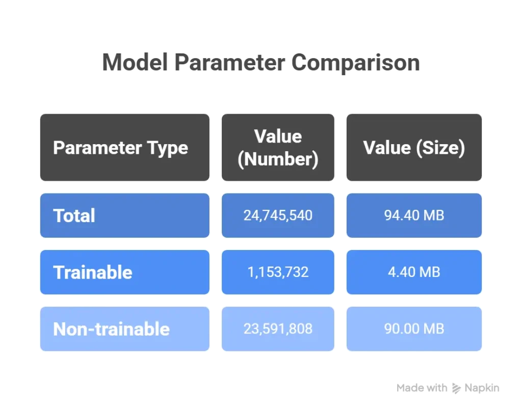
ResNet50 already learned useful visual features from ImageNet. We freeze its layers so we don’t retrain millions of weights on our small dataset. This speeds training and reduces overfitting. We only train a compact head on top to specialize in cars.
Add a compact head (how it helps)
The head learns car-specific patterns while staying regularized:
- BatchNormalization stabilizes activations.
- Dense(512, ReLU, L2) adds learning capacity with weight decay.
- Dropout(0.6) fights overfitting.
- Dense(len(classes), softmax) outputs probabilities for our classes list.
Loss + optimizer (stable training)
We use categorical cross-entropy with label smoothing (0.1) so the model doesn’t get over-confident, and Adam with a modest learning rate to update the new head smoothly.
from tensorflow.keras.applications.resnet50 import ResNet50
from tensorflow.keras.layers import Dense, Dropout, BatchNormalization
from tensorflow.keras.models import Model
from tensorflow.keras.regularizers import l2

# 1) Load ResNet50 without its original classifier (top) and with global average pooling.
base = ResNet50(
    weights='imagenet',
    include_top=False,
    pooling='avg',
    input_shape=(224, 224, 3)
)

# 2) Freeze all backbone layers: reuse generic vision features, avoid overfitting.
for layer in base.layers:
    layer.trainable = False

# 3) Add a small classification head to specialize on car models.
x = base.output                     # shape: (None, 2048) after global average pooling
x = BatchNormalization()(x)         # stabilize activations for faster, steadier training
x = Dense(512, activation='relu',   # capacity to learn car-specific features
          kernel_regularizer=l2(5e-4))(x)  # L2 (weight decay) to reduce overfitting
x = Dropout(0.6)(x)                 # randomly drop 60% units during training -> robustness
output = Dense(len(classes),        # number of car classes (196 for Stanford Cars)
               activation='softmax',
               kernel_regularizer=l2(5e-4))(x)

model_untrained = Model(inputs=base.input, outputs=output)

# Optional: confirm backbone is frozen and head is trainable.
model_untrained.summary()

# 4) Compile with label smoothing to prevent over-confidence on fine-grained classes.
from tensorflow.keras.optimizers import Adam
from tensorflow.keras.losses import CategoricalCrossentropy

model_untrained.compile(
    optimizer=Adam(learning_rate=0.001),                 # modest LR for stable updates
    loss=CategoricalCrossentropy(label_smoothing=0.1),   # smoother, better generalization
    metrics=['accuracy']
)
👉 The architecture of a model really matters, it’s the blueprint that decides how well the model can learn. The choices we made here (freezing ResNet50, adding BatchNorm, dropout, and dense layers) will directly affect whether the model simply memorizes the training images or truly learns to recognize car models. And in practice, this can often be a process of trial and error, testing different setups to see how each one impacts training.
Right now, what we have is an untrained model. It’s just the frozen ResNet50 backbone plus our new head (changed to output 196 classes instead of the original 1,000 classes from ImageNet). But the head’s weights are still random. If we tested it at this stage, the predictions would be very poor, essentially just random guesses across 196 possibilities (around 0.005).
We’ll use this as a quick demonstration: first, we’ll test the untrained model to see how bad the predictions are, and then we’ll train it properly (using transfer learning without fine-tuning) to show how much better the outcomes can become.
Also, you might have noticed we introduced several technical terms along the way, like dropout, label smoothing, backbone, optimizer, and more. If any of these sound unfamiliar, you can check out my post AI & Machine Learning Glossary: Common Terms Beginners Should Know where I explain these concepts in simple language.
Testing the Untrained Model
Before we train, let’s see how our model performs in its current state. With 196 classes, a random guess would lead to an accuracy of about 0.005 (half a percent). When we actually evaluate our untrained model on the validation set, the accuracy comes out at 0.0037 — basically random guessing, just as expected.
# --- Evaluate the model on the validation set before any training ---
# Since the classification head is still untrained (random weights),
# we expect the accuracy to be around random guessing (≈1/196 ≈ 0.005).

loss, acc = model_untrained.evaluate(validation_generator, verbose=1)
print(f"Pre-training accuracy: {acc:.4f}")
To make this more concrete, we can also look at a few sample images from the validation set. For each image, we display the true label (T) and the predicted label (P) from our untrained model. As you’ll see, the predictions are completely off at this stage — confirming that the head is still random and hasn’t learned anything yet.
Training the Model
Time to teach our new head to “speak car.” We’ll run training with a few helpers (callbacks) to keep it efficient and stable, then record how long it took and which epoch was best.
What the callbacks do
- EarlyStopping: watches validation loss. If it stops improving, we stop and restore the best weights.
- ReduceLROnPlateau: when progress stalls, lower the learning rate so the model can squeeze out a bit more validation gain.
- ModelCheckpoint: saves the single best model file to disk.
- CSVLogger: writes a row per epoch to
train_log.csvfor plots and reproducibility.
Train, time it, and summarize
We run up to 100 epochs (it may stop earlier), then print total time and the best epoch’s metrics.
import time, numpy as np
from tensorflow.keras.callbacks import EarlyStopping, ReduceLROnPlateau, ModelCheckpoint, CSVLogger

cb = [
    EarlyStopping(monitor='val_loss', patience=8, min_delta=1e-3, restore_best_weights=True),
    ReduceLROnPlateau(monitor='val_loss', factor=0.2, patience=3, cooldown=1, min_lr=1e-6, verbose=1),
    ModelCheckpoint('tl_best.keras', monitor='val_loss', mode='min', save_best_only=True),
    CSVLogger('train_log.csv', append=False),
]

t0 = time.perf_counter()
history = model_untrained.fit(
    train_generator,
    validation_data=validation_generator,
    epochs=100,
    callbacks=cb,
    verbose=1
)
total_sec = time.perf_counter() - t0

# Best epoch summary (by lowest val_loss) + timing
epochs_run   = len(history.history["loss"])
best_idx     = int(np.argmin(history.history["val_loss"]))
best_val_acc = history.history["val_accuracy"][best_idx]
best_val_loss= history.history["val_loss"][best_idx]

print(f"[Time] Total: {total_sec/60:.2f} min | Avg/epoch: {total_sec/epochs_run:.1f} s")
print(f"[Best] Epoch {best_idx+1} | val_acc={best_val_acc:.4f} | val_loss={best_val_loss:.4f}")
Why this setup works
- Monitoring validation loss avoids chasing noisy accuracy swings.
- EarlyStopping + Checkpoint prevents over-training and keeps the best model.
- LR reduction often unlocks a small late-stage improvement.
- Timing info gives you concrete numbers for the blog (total minutes and avg seconds/epoch).
Training Curves: Spotting Overfitting
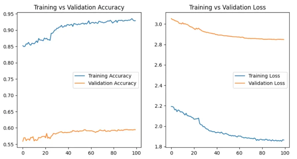
Here’s where things get interesting. When we look at the curves, the training accuracy shoots up close to 95%, while the validation accuracy stalls around 60%. That gap is what we call overfitting.
So what does overfitting really mean? Imagine a student who memorizes every answer in the practice book. On the day of the exam, if the questions are worded a little differently, the student struggles. The same thing happens here: the model is getting too good at recognizing the exact training images, but it fails to generalize to new, unseen ones (our validation set).
Why is that bad? Because in the real world, the goal isn’t to ace the training set, it’s to correctly classify cars it has never seen before. A model that only memorizes won’t be useful outside the lab.
That’s why we added tricks like dropout, L2 regularization, label smoothing, and augmentation, they force the model to learn more general patterns instead of just memorizing. They help, but as the curves show, there’s still a clear gap.
The big takeaway: high training accuracy is meaningless if validation accuracy doesn’t follow along. What matters most is how well the model handles new data.
Conclusion & Next Steps
So, what did we learn? Starting from an untrained head, our model was basically guessing. After training with transfer learning, we reached around 55% validation accuracy on a tough fine-grained dataset. That shows the power of reusing ResNet50’s ImageNet knowledge.
But as the curves revealed, we’re still fighting overfitting. The model gets close to perfect on the training set, while validation lags behind. To push further, we can keep trying different tricks:
- stronger or weaker dropout
- adjusting L2 regularization
- experimenting with data augmentation
- playing with batch size and learning rate schedules
- or even early stopping patience
All of these can help a little, but there’s a bigger step: fine-tuning.
What’s fine-tuning, and how is it different?
- Transfer learning (what we did here): freeze the backbone and only train the new head. This is fast and works well when the dataset is small.
- Fine-tuning: unfreeze part (or all) of the backbone and train it at a very low learning rate. This lets the model adapt its deeper features to the new dataset instead of relying only on the head.
Fine-tuning usually gives a significant boost on fine-grained datasets like Stanford Cars, but it also needs more compute and careful tuning to avoid overfitting.
👉 In a future post, we’ll dive into fine-tuning ResNet50 on the same dataset, show how it differs from plain transfer learning, and see how much improvement it brings. I’ll update this post with the link when it’s ready.
Want to Learn More or Have Questions?
📩 For any inquiries, contact me here.
📚 Explore more tutorials and guides in the Blog section.

