Introduction
Ready to dive into machine learning? Let’s build a simple ML model from scratch using Python! In this step-by-step guide, we’ll train a classifier to recognize different types of iris flowers using the famous Iris dataset.
This dataset includes measurements like sepal length, sepal width, petal length, and petal width for three species: Setosa, Versicolor, and Virginica. Our goal? Train a model that can predict a flower’s species based on these measurements.
We’ll walk through the entire process in three parts:
- Part 1: Loading and exploring the dataset
- Part 1: Preparing the data for training
- Part 2: Training a classifier with scikit-learn
- Part 3: Evaluating the model’s performance
- Part 3: Making predictions on new data
If some of these steps sound unfamiliar, don’t worry! We’ll break everything down along the way. By the end of this guide, you’ll have built and run your first machine learning project while understanding the essential ML workflow.
By the end of this part, you’ll be ready for Model Training.
Before You Start
Make sure your Python environment is set up with libraries like pandas, matplotlib, and scikit-learn (refer to Getting Started with Python for Machine Learning for setup details).
1. Step 1: Select and Understand the Dataset
For this beginner-friendly project, we’re using the Iris dataset, a small and well-known dataset often considered the “Hello World” of machine learning.
It contains measurements for three species of iris flowers:
🌸 Setosa
🌿 Versicolor
🌼 Virginica
Each flower is described by four measurements:
- Sepal length
- Sepal width
- Petal length
- Petal width
1.1 How Our Model Will Learn
The idea behind our model is simple:
Each species has a unique pattern of measurements, and our model will learn to classify a flower based on these differences.
For example:
- Setosa → Short petals, small sepals
- Versicolor → Medium-sized petals, moderate sepals
- Virginica → Long petals, large sepals
If we look at petal length vs. petal width, we can see that each species clusters in a different area.
let’s first look at the final outcome of a scatter plot showing how the species group together based on their petal measurements:
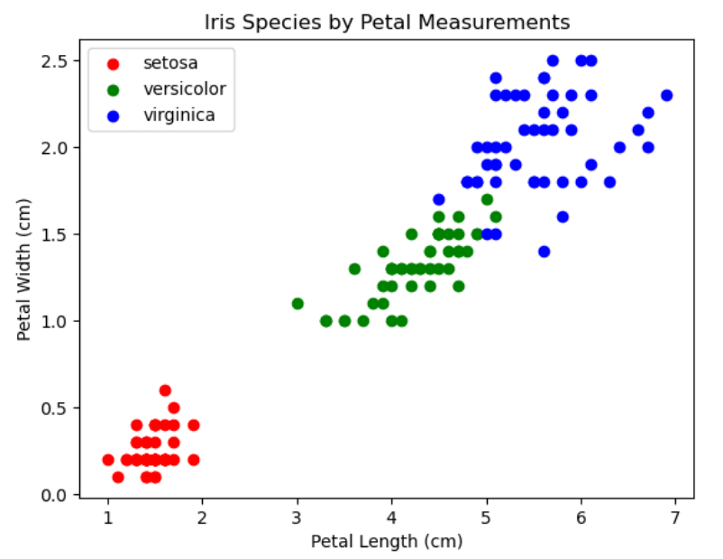
🔴 Setosa (Red): Clearly separated with shorter and narrower petals
🟢 Versicolor (Green) → Overlaps slightly but has medium-sized petals
🔵 Virginica (Blue) → Has longer and wider petals
1.2 Final Outcome of This Step
✅ We understand how the model will classify flowers based on measurements.
✅ We visualized how each species forms a pattern in measurement space.
✅ We see that petal length & width are key features for classification.
2. Step 2: Loading the Dataset
Now that we understand the structure of the dataset and how our model will learn, let’s bring the data into Python so we can start working with it.
Luckily, scikit-learn provides the Iris dataset for us, so we can load it directly—no need to download anything separately.
Here’s how we load the dataset using scikit-learn:
from sklearn.datasets import load_iris

# Load the Iris dataset
iris = load_iris()

# Print basic details
print("Feature names:", iris.feature_names)
print("Target classes:", iris.target_names)
print("First data point:", iris.data[0], "->", iris.target_names[iris.target[0]])
2.1 Understanding the Data Output
When we run this, we get:
- Feature names
['sepal length (cm)', 'sepal width (cm)', 'petal length (cm)', 'petal width (cm)']
- Target classes
['setosa', 'versicolor', 'virginica']
- First data point
[5.1 3.5 1.4 0.2] -> setosa
This tells us that the first flower in the dataset has relatively small petals and belongs to the Setosa species.
2.2 Visualizing the Data Structure
Now, let’s break down the dataset into a table format to see how it looks:
Sepal
Length (cm) | Sepal
Width (cm) | Petal
Length (cm) | Petal
Width (cm) | Species |
5.1 | 3.5 | 1.4 | 0.2 | Setosa |
4.9 | 3.0 | 1.4 | 0.2 | Setosa |
7.0 | 3.2 | 4.7 | 1.4 | Versicolor |
6.3 | 3.3 | 6.0 | 2.5 | Virginica |
- Each row represents a flower, with its measurements.
- The Species column tells us which type of flower it is.
- Setosa has much smaller petal measurements than Virginica, confirming what we saw earlier in the scatter plot.
2.3 Final Outcome of This Step
✅ We successfully loaded the dataset into Python.
✅ We understand how the data is structured (features & labels).
✅ We see that each species has a unique range of measurements.
Now that our dataset is loaded, let’s explore it further to find patterns that can help our model learn.
3. Step 3: Exploratory Data Analysis (EDA)
Before training our model, let’s take a deeper look at the dataset. This step, called Exploratory Data Analysis (EDA), helps us understand patterns, relationships, and potential challenges in our data.
3.1 Checking the Dataset Structure
First, let’s inspect the dataset to see how many samples and features we have. We’ll also convert it into a pandas DataFrame for easier exploration.
import pandas as pd
import matplotlib.pyplot as plt
from sklearn.datasets import load_iris

# Load the Iris dataset
iris = load_iris()

# Convert to a DataFrame
df = pd.DataFrame(iris.data, columns=iris.feature_names)
df['species'] = iris.target  # Add species labels

# Map numeric species labels to actual names
df['species'] = df['species'].map({0: 'setosa', 1: 'versicolor', 2: 'virginica'})

# Display dataset shape and first few rows
print("Dataset shape:", df.shape)
print(df.head())

# Show summary statistics
df.describe()
Key Outputs:
Dataset shape: (150, 5)→ 150 flowers, each with 4 features + species labeldf.head()→ Displays the first five rowsdf.describe()→ Shows summary statistics
3.2 Visualizing the Data: Petal Length vs. Petal Width
Since we are trying to classify species based on measurements, let’s plot a scatter plot showing the relationship between petal length and petal width.
# Scatter plot: Petal length vs. Petal width
colors = {'setosa': 'red', 'versicolor': 'green', 'virginica': 'blue'}
for species, color in colors.items():
    subset = df[df['species'] == species]
    plt.scatter(subset['petal length (cm)'], subset['petal width (cm)'],
                c=color, label=species)

plt.xlabel('Petal Length (cm)')
plt.ylabel('Petal Width (cm)')
plt.legend()
plt.title('Iris Species by Petal Measurements')
plt.show()
3.3 Final Outcome of This Step
✅ We explored the dataset and checked its structure.
✅ We plotted the data, showing that petal length & width are useful for classification.
✅ We examined summary statistics, confirming Setosa is easily distinguishable, while Versicolor & Virginica overlap slightly.
What’s Next?
Congratulations! You’ve successfully prepared your dataset for training your first machine learning model in Python. But how can we train the model?
In Part 2, we’ll train the model, understand steps for model trainign and use it to make predictions in later stages.
Read the next part here: Building Your First Machine Learning Model in Python: Model Training