Table of Contents
ToggleIntroduction
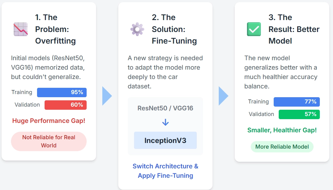
In our last post, we applied Transfer Learning to the Stanford Cars dataset using the ResNet50 model. While this gave us a good starting point, the model showed clear signs of overfitting: high accuracy on the training data, but a much lower accuracy on new, unseen images.
To see if another architecture would help, I also ran some offline tests with the VGG16 model, but the story was much the same, it also struggled to generalize. When a model cannot perform well on new data, it is not reliable for real-world tasks.
To improve our results, we need a better strategy.In this guide, we will explore a new approach. We are switching to the InceptionV3 architecture and introducing a more advanced technique called Fine Tuning. This process allows us to more deeply adapt the pretrained model to the specific features of our car images, aiming to close the gap between training and validation accuracy.
This step-by-step tutorial documents our complete workflow for Fine Tuning. The goal is to build a more robust car recognition model that truly learns, and the methods you learn here can be adapted for any custom image classification project you want to build.
By the end, you will:
- Understand the core concept of Fine Tuning.
- Build a model with InceptionV3 ready for Fine Tuning.
- Use a two-phase training strategy for effective Fine Tuning.
- Learn how to unfreeze layers for the second stage of training.
- Evaluate your model’s performance after Fine Tuning.
Environment and Dataset Setup
In our previous post, we introduced the Stanford Cars dataset and walked through the detailed process of exploring its structure and splitting it into training, validation, and test sets. If you are starting from scratch, we recommend following that guide first to get your data organized.
For this post, we will assume you have the dataset ready in three separate folders:
train, validation, and test.
Data Preprocessing and Augmentation
The steps we take here will look very familiar if you read our last post. We are following the same core strategy of preprocessing and augmenting our data. However, we will make a few key adjustments to meet the specific requirements of our new model, InceptionV3.
The two main processes are:
- Preprocessing: Just like ResNet50, InceptionV3 was trained on the ImageNet dataset and requires a specific input format. We will use its dedicated
preprocess_inputfunction to make sure our images are scaled correctly. - Augmentation: To help our model generalize better and avoid overfitting, we will apply random transformations (like rotating and flipping) to our training images.
Step 1: Set Image Size and Batch Size
Here, we will define our core parameters. The most important change from our last post is the image size. InceptionV3 was designed to work with larger images than ResNet50.
- Image Size: All images will be resized to 299 × 299 pixels. This is the standard input size for the InceptionV3 architecture.
- Batch Size: We will stick with a batch size of 32, which is a good balance for most GPUs.
- Seed: We set a random seed to ensure our results are reproducible.
from tensorflow.keras.preprocessing.image import ImageDataGenerator
from tensorflow.keras.applications.inception_v3 import preprocess_input

IMG_SIZE = (299, 299) # Updated for InceptionV3
BATCH_SIZE = 32 # Keep for now, but be prepared to lower it if you get a memory error
SEED = 42
Step 2: Define the Training Data Generator
Next, we set up the ImageDataGenerator for our training set. This Keras utility will load images from our directory and apply our chosen transformations in real-time. This means the model sees slightly different versions of the images in each epoch, which is great for learning.
train_datagen = ImageDataGenerator(
preprocessing_function=preprocess_input,
horizontal_flip=True,
rotation_range=10,
width_shift_range=0.1,
height_shift_range=0.1,
zoom_range=(0.95, 1.05),
shear_range=0.1,
brightness_range=(0.85, 1.15),
channel_shift_range=1.0,
fill_mode='reflect'
)
Step 3: Validation and Test Generators
For the validation and test sets, we only apply the necessary preprocessing. We do not use any random augmentation here because we need an honest, unbiased measure of our model’s performance on the clean, original images.
val_test_datagen = ImageDataGenerator(
preprocessing_function=preprocess_input
)
Step 4: Create Generators for Each Split
Finally, we connect our generators to the image folders on our disk using the flow_from_directory method. Keras automatically handles the labeling based on the subdirectory names.
Note: Remember to replace the placeholder paths and define the classes variable according to your project setup.
# Assuming 'train_data_dir', 'validation_data_dir', 'test_data_dir',
# and 'classes' are defined from your dataset preparation step.

train_generator = train_datagen.flow_from_directory(
directory=train_data_dir, target_size=IMG_SIZE, batch_size=BATCH_SIZE,
classes=classes, class_mode='categorical', shuffle=True, seed=SEED
)

validation_generator = val_test_datagen.flow_from_directory(
directory=validation_data_dir, target_size=IMG_SIZE, batch_size=BATCH_SIZE,
classes=classes, class_mode='categorical', shuffle=False
)

test_generator = val_test_datagen.flow_from_directory(
directory=test_data_dir, target_size=IMG_SIZE, batch_size=BATCH_SIZE,
classes=classes, class_mode='categorical', shuffle=False
)

Data Preparation & Workflow Overview
Now we have our dataset ready and organized into training, validation, and test folders. We applied the required preprocessing for InceptionV3 using its preprocess_input function and set the image size to 299×299. To improve generalization, we created a training generator with augmentation techniques like flips, shifts, rotations, and brightness changes. For validation and test sets, we kept only preprocessing to ensure unbiased evaluation. Finally, we connected all three splits to Keras generators, giving us a clean and reproducible pipeline to feed images into our model.
In simple terms, we resized all images to the format InceptionV3 expects, applied some random changes to the training images so the model doesn’t just memorize them, and kept the validation and test images clean so they reflect real-world performance. Finally, we linked everything to Keras generators, which act like pipelines that automatically feed the right data to our model during training.
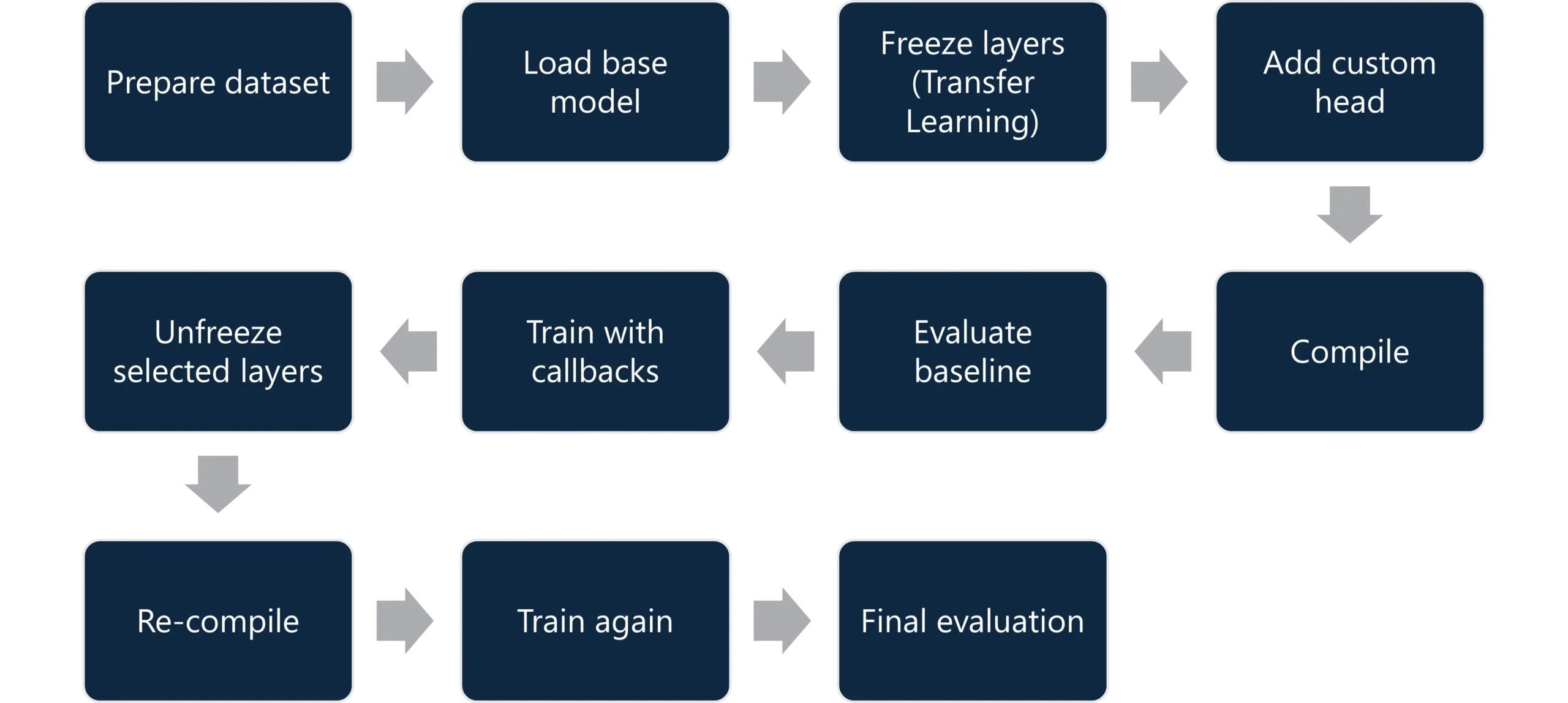
With the data pipeline ready, the overall fine-tuning workflow looks like this:
Building the Model
With our data pipeline ready, the next step is to design the model itself. We’ll start by loading the InceptionV3 architecture pretrained on ImageNet. Instead of using the full model, we’ll exclude its top layers so we can add our own custom classification head later.
Load the InceptionV3 Base Model
from tensorflow.keras.applications.inception_v3 import InceptionV3
from tensorflow.keras.layers import Dense, Dropout, BatchNormalization, Activation, GlobalAveragePooling2D
from tensorflow.keras.models import Model
from tensorflow.keras.regularizers import l2

# Load the InceptionV3 base model
base = InceptionV3(
    weights='imagenet',      # Start with pretrained ImageNet weights
    include_top=False,       # Exclude the default fully connected layers
    input_shape=(299, 299, 3) # Input size expected by InceptionV3
)
Loading InceptionV3 with weights='imagenet', include_top=False, and input_shape=(299, 299, 3) means we start with pretrained features, drop the default classifier, and set the input size for our dataset.
Freeze the Base Model
# Freeze all layers in the base model
for layer in base.layers:
    layer.trainable = False
Freezing means the pretrained weights won’t change during training, so the model keeps its learned ImageNet features while we train only the new custom layers.
Add a Custom Classification Head
Now that we have the InceptionV3 base model ready and frozen, we need to attach a new “head” on top. The original head was built for 1,000 ImageNet classes, but here we replace it with layers suited for our 196 car classes. This custom head combines pooling, dense layers, normalization, dropout, and finally a softmax output layer.
# Custom head with GlobalAveragePooling2D
x = base.output                              # take feature maps from InceptionV3
x = GlobalAveragePooling2D()(x)               # pool H×W features to a single vector
x = Dense(512, kernel_regularizer=l2(1e-3))(x) # dense layer with L2 weight decay
x = BatchNormalization()(x)                   # stabilize/accelerate training
x = Activation('relu')(x)                     # non-linearity
x = Dropout(0.5)(x)                           # reduce overfitting

x = Dense(256, kernel_regularizer=l2(1e-3))(x) # second dense block (smaller)
x = BatchNormalization()(x)
x = Activation('relu')(x)
x = Dropout(0.5)(x)

output = Dense(len(classes), activation='softmax',
               kernel_regularizer=l2(1e-3))(x) # class probabilities

# Final model (base + custom head)
model_untrained = Model(inputs=base.input, outputs=output)
GlobalAveragePooling2D
After the base model, we get many feature maps (grids of numbers showing patterns). Flattening them would create too many parameters. GlobalAveragePooling2D instead averages each map into a single value, keeping the signal but cutting complexity.
💡Think of it as looking at all a student’s quiz results and writing down just the average score for the subject. You lose the tiny details of each quiz, but you get a clear measure of overall performance. This way, the record is shorter (fewer numbers), easier to compare, and less likely to be biased by one unusually high or low result.
Dense Layer
A Dense layer is a fully connected layer where every input connects to every output. It learns patterns by combining the signals from the features that come before it.
💡Think of it as the final exam that combines all quizzes from every subject. It pulls together all the small pieces of knowledge into one big decision. This gives the model the power to recognize more complex patterns, just like an exam shows the student’s overall understanding.
Kernel Regularizer (L2)
The L2 regularizer adds a small penalty to large weights, preventing the model from relying too heavily on any single connection.
💡Think of it as a teacher who tells students not to memorize one tricky question but to balance their effort across the whole subject. This keeps the model fair, balanced, and better at generalizing to new data.
BatchNormalization
This layer normalizes outputs so they stay in a stable range, helping the network train faster and more reliably.
💡Think of it as adjusting all students’ scores to the same scale (like converting grades from 0–20 to percentages). It makes comparing easier, prevents extremes from causing issues, and keeps learning smooth.
Activation (ReLU)
ReLU (Rectified Linear Unit) turns negative values into zero while keeping positive ones. This non-linearity allows the model to learn more complex patterns.
💡Think of it as filtering out wrong answers and only keeping useful ones. This keeps the system simple, avoids wasting energy on negatives, and focuses on the signals that matter.
Dropout
Dropout randomly turns off some neurons during training so the model doesn’t rely on the same paths every time.
💡Think of it as a teacher who sometimes hides certain practice questions so students can’t memorize them. This forces them to study broadly, making them stronger and more adaptable.
Second Dense Block
Adding another Dense block gives the model more learning capacity but with fewer neurons, making it efficient and reducing overfitting.
💡Think of it as giving students a second, smaller test after the big exam. It reinforces learning without overwhelming them, ensuring they truly understand.
Output Layer (Dense + Softmax)
The final Dense layer has as many outputs as classes, and Softmax converts these into probabilities that sum to 1.
💡Think of it as the final report card. After all exams and tests, the school lists the probability of each student belonging to a particular grade level. It’s clear, interpretable, and gives one confident answer.
Compile the Model
After building the architecture, we need to “compile” the model — this sets the optimizer, loss function, and metrics that will guide training.
from tensorflow.keras.optimizers import Adam
from tensorflow.keras.losses import CategoricalCrossentropy
from tensorflow.keras.metrics import TopKCategoricalAccuracy

model_untrained.compile(
    optimizer=Adam(learning_rate=3e-4),                # optimizer controls weight updates
    loss=CategoricalCrossentropy(label_smoothing=0.1), # loss measures prediction error
    metrics=['accuracy', TopKCategoricalAccuracy(k=3)] # metrics track performance
)
Optimizer (Adam)
The optimizer controls how the model updates its weights while learning. Adam is a good choice because it adjusts the updates automatically, helping the model learn faster and more reliably.
Learning Rate (3e-4)
The learning rate sets how big each learning step is. If it’s too high, the model might skip over the right answer; if it’s too low, training becomes very slow. Here we use 3e-4, which is a safe middle value.
Loss Function (Categorical Crossentropy)
The loss function measures how far the model’s predictions are from the correct answers. Categorical crossentropy is made for problems where we pick one class out of many, which fits our 196 car types.
Label Smoothing (0.1)
Label smoothing slightly softens the “correct answer” labels. This stops the model from being too confident and helps it perform better on new data.
Metric (Accuracy)
Accuracy shows how many predictions were correct out of all attempts. It’s the simplest way to track progress while training.
Metric (Top-K Accuracy, k=3)
Top-K accuracy checks if the correct class is within the top 3 predictions. This is useful when there are many classes and the model’s best guess might not always be the first one.
Baseline Test with Pretrained InceptionV3
Before training our custom head, we tested the pretrained InceptionV3 model to see how well it could classify car images without any fine-tuning. The results were very poor, as expected, since the model was trained on ImageNet and not on the specific car types in the Stanford Cars dataset. The model might recognize that the object is a car rather than a chair, but it cannot tell which exact make or model the car is.
Results:
- Pre-training accuracy: 0.37%
- Pre-training Top-3 accuracy: 1.21%
The image below shows some sample predictions. Notice that the model’s guesses (P:) do not match the true car labels (T:). This highlights why transfer learning and fine-tuning are necessary, the base model alone cannot handle our specific dataset.

Training with Callbacks
We have now built and compiled our model, tested the pretrained base, and we are ready to start training. But training deep models can take a lot of time, and without proper checks we may either overfit or waste resources on unnecessary epochs. To make training more efficient and reliable, we will define a set of callbacks, small helpers that monitor progress and adjust training automatically.
At this point, we are training only the custom head while keeping the InceptionV3 base frozen. This is the Transfer Learning (TL) stage, not yet Fine Tuning.
from tensorflow.keras.callbacks import EarlyStopping, ReduceLROnPlateau, ModelCheckpoint, CSVLogger

cb_TL = [
    EarlyStopping(monitor='val_loss', mode='min', patience=5, min_delta=5e-4, restore_best_weights=True),
    ReduceLROnPlateau(monitor='val_loss', mode='min', factor=0.5, patience=3, cooldown=1, min_lr=1e-6, verbose=1),
    ModelCheckpoint('tl_best.keras', monitor='val_loss', mode='min', save_best_only=True),
    CSVLogger('train_log.csv', append=False),
]
- EarlyStopping: stops training if validation loss doesn’t improve for a set number of epochs.
→ Prevents wasting time and avoids overfitting. - ReduceLROnPlateau: lowers the learning rate if progress stalls.
→ Helps the model fine-tune better when it gets stuck. - ModelCheckpoint: saves the best version of the model during training.
→ Ensures we keep the best weights, not just the last ones. - CSVLogger: saves training history (loss, accuracy, etc.) into a CSV file.
→ Makes it easy to analyze results later.
Training the Model (Transfer Learning)
With the callbacks ready, we can now train the model. In this phase, only the custom head is being trained, while the InceptionV3 base remains frozen. We train for up to 100 epochs, but thanks to EarlyStopping, the process will stop once validation loss stops improving.
import time, numpy as np

# Start a timer to measure how long training takes
t0 = time.perf_counter()

# Train the model
# - train_generator provides training images with augmentation
# - validation_generator provides clean validation images
# - epochs=100 is just a maximum, EarlyStopping will stop earlier if needed
# - callbacks=cb_TL ensures training is monitored and adjusted automatically
history = model_untrained.fit(
    train_generator,
    validation_data=validation_generator,
    epochs=100,       # maximum number of epochs
    callbacks=cb_TL,  # our callback list (early stopping, checkpoints, etc.)
    verbose=1         # show training progress in the console
)

# Measure total training time
total_sec = time.perf_counter() - t0

# Number of epochs actually run (before EarlyStopping stopped)
epochs_run = len(history.history["loss"])

# Find the epoch with the lowest validation loss
best_idx = int(np.argmin(history.history["val_loss"]))

# Extract the validation metrics at that best epoch
best_val_acc = history.history["val_accuracy"][best_idx]
best_val_loss = history.history["val_loss"][best_idx]
best_val_top3_acc = history.history["val_top_k_categorical_accuracy"][best_idx]

# Print summary of training results
print(f"[Time] Total: {total_sec/60:.2f} min | Avg/epoch: {total_sec/epochs_run:.1f} s")
print(f"[Best] Epoch {best_idx+1} | val_loss={best_val_loss:.4f} | "
      f"val_acc={best_val_acc:.4f} | val_top3_acc={best_val_top3_acc:.4f}")
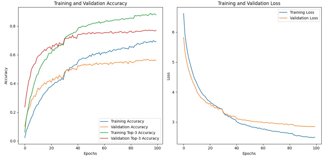
After training, the model showed clear improvements compared to the baseline test. The validation accuracy reached 56.4%, and the Top-3 accuracy reached 76.5%. Training took about 273 minutes in total (over 4.5 hours), averaging 164 seconds per epoch, with the best performance recorded at epoch 99.
This is a big step forward from the pretrained model’s 0.37% accuracy and 1.21% Top-3 accuracy, proving that even with the base layers frozen, the custom head can already learn meaningful patterns from the car images.
The plots below show the training and validation accuracy (left) and the loss (right) over the epochs. We can see a steady improvement, with validation accuracy stabilizing around 56% and Top-3 accuracy reaching about 76%. The loss curves also show a consistent downward trend, with validation loss closely following training loss, which means the model is learning effectively without severe overfitting.
Training the Model (Fine Tuning)
Now we switch from Transfer Learnign to Fine Tuning: load the best transfer learning checkpoint, partially unfreeze the base, compile with a much smaller LR, and train again.
Load the best Transfer Learning (TL) model
We continue from the strongest TL weights instead of starting over.
from tensorflow.keras.models import load_model

# Load the best model from the transfer learning phase
model_ft = load_model('tl_best.keras')
Unfreeze selected layers
We fine-tune only the deeper layers (more task-specific features) to avoid overfitting and keep training stable.
# Unfreeze the base model
model_ft.trainable = True

# Keep early layers frozen; unfreeze only the later blocks
# (example: unfreeze the last 23 layers)
for layer in model_ft.layers[:249]:
    layer.trainable = False

model_ft.summary()
Re-compile with a smaller LR
Fine tuning uses tiny updates so we don’t overwrite useful pretrained representations.
from tensorflow.keras.optimizers import Adam
from tensorflow.keras.losses import CategoricalCrossentropy
from tensorflow.keras.metrics import TopKCategoricalAccuracy

model_ft.compile(
    optimizer=Adam(learning_rate=5e-7),            # very small steps to preserve pretrained features
    loss=CategoricalCrossentropy(label_smoothing=0.1),
    metrics=['accuracy', TopKCategoricalAccuracy(k=3)]
)
Train (Fine Tuning)
We train longer with safeguards (callbacks)
import time, numpy as np

print("Starting Fine-tuning...")

t0 = time.perf_counter()
history_ft = model_ft.fit(
    train_generator,
    validation_data=validation_generator,
    epochs=150,
    callbacks=cb_TL,   # reuse the same callbacks
    verbose=1
)
total_sec = time.perf_counter() - t0

epochs_run = len(history_ft.history["loss"])
best_idx = int(np.argmin(history_ft.history["val_loss"]))
best_val_acc = history_ft.history["val_accuracy"][best_idx]
best_val_loss = history_ft.history["val_loss"][best_idx]
best_val_top3_acc = history_ft.history["val_top_k_categorical_accuracy"][best_idx]

print(f"[Time] Total: {total_sec/60:.2f} min | Avg/epoch: {total_sec/epochs_run:.1f} s")
print(f"[Best] Epoch {best_idx+1} | val_loss={best_val_loss:.4f} | val_acc={best_val_acc:.4f} | val_top3_acc={best_val_top3_acc:.4f}")
After fine-tuning, the model achieved a small but meaningful improvement compared to the transfer learning phase. The validation accuracy increased to 57.3%, and the Top-3 accuracy reached 77.4%, with validation loss dropping to 2.80. Training was much faster this time, taking only 38 minutes in total, averaging 144 seconds per epoch, with the best performance recorded at epoch 11.
These results show that carefully unfreezing part of the InceptionV3 base and training with a very low learning rate helps the model capture finer details, pushing accuracy beyond what the frozen base alone could achieve.
The plots below show the combined training curves. The red dotted line marks the start of fine-tuning. After this point, validation accuracy and Top-3 accuracy both rise slightly, while validation loss decreases further, confirming the benefit of this additional training phase.
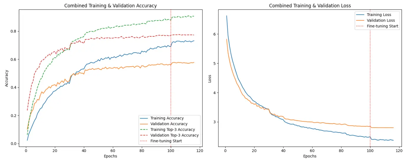
The improvements from fine-tuning are only slight compared to transfer learning. In practice, TL was already doing most of the heavy lifting. This happens because the Stanford Cars dataset is relatively small and InceptionV3’s pretrained features are already strong and general enough to capture most patterns. Once the custom head was trained, the base model didn’t need much extra adjustment. Fine-tuning gave a marginal boost, but TL alone might be sufficient for many real-world use cases where time and resources are limited.
Qualitative Results: Model Predictions After Training
To better illustrate the improvement, we tested the trained model on car images and compared the predictions. Unlike the baseline test (where predictions were almost entirely wrong), the model now correctly classifies most examples. The green labels show correct matches between the true class (T:) and the predicted class (P:), while the few errors are marked in red. This practical view highlights how Transfer Learning and Fine Tuning transformed the pretrained InceptionV3 from a generic feature extractor into a car recognition model that works reliably.

Testing on a New, Unseen Car Image
To evaluate how well the model generalizes, we tested it on a car image taken from the internet, one that was not part of the Stanford Cars dataset.

The model produced the following predictions:
Top 5 Predictions:
Hyundai Elantra Sedan 2007 (Confidence: 79.99%) Correct
Chevrolet Malibu Sedan 2007 (Confidence: 1.89%)
Hyundai Sonata Hybrid Sedan 2012 (Confidence: 1.86%)
Ford Focus Sedan 2007 (Confidence: 1.37%)
Hyundai Sonata Sedan 2012 (Confidence: 1.31%)
The true label of the car was Hyundai Elantra Sedan 2007, which the model predicted correctly with ~80% confidence. This shows that the fine-tuned model is not only effective on the Stanford Cars dataset but also capable of handling real-world images outside the training data.
Results Comparison at a Glance
The table below summarizes all phases; baseline, transfer learning, and fine tuning. It clearly shows how transfer learning brought the biggest jump in performance, while fine tuning added only a small improvement.

Conclusion & Next Steps
In this guide, we started with a pretrained InceptionV3 model that could barely recognize car types, achieving only 0.37% accuracy. By applying Transfer Learning, we boosted performance dramatically to 56.4% accuracy and 76.5% Top-3 accuracy. Adding Fine Tuning nudged the results slightly higher to 57.3% accuracy and 77.4% Top-3 accuracy, showing that most of the benefit came from transfer learning, with fine tuning adding only minor gains.
This experiment highlights two important lessons:Transfer Learning is powerful, even with a frozen base model, pretrained features can adapt to new datasets quickly.
Fine Tuning adds incremental improvements, but may not always be worth the extra complexity unless very high accuracy is needed.
Next steps:
Try different architectures (EfficientNet, ResNet101, etc.) for comparison.
Explore stronger augmentation to reduce overfitting.
Evaluate on more external images to test generalization.
Deploy the trained model into a simple web app or API to make it usable in real-world scenarios.
By combining transfer learning with careful fine tuning, you now have a strong baseline for building car recognition systems, and the same workflow can be applied to many other image classification tasks.
Want to Learn More or Have Questions?
📩For any inquiries, contact me here.
📚 Explore more tutorials and guides in the Blog section.

