Table of Contents
ToggleIntroduction
LoL match prediction using machine learning is more fun than you think! In this guide, we’ll use logistic regression and PyTorch to predict match outcomes based on in-game stats.
In this beginner-friendly post, you’ll learn how to use logistic regression, a simple yet powerful machine learning method, to predict match results using PyTorch.
We’ll keep things straightforward, and by the end, you’ll understand:
- How logistic regression works for predicting match outcomes.
- How to interpret results to see what influences wins or losses.
- The practical limits of this method and what alternatives exist.
Ready to dive into predicting League of Legends outcomes? Let’s start exploring!
1. Understanding the Data
Before building our model, let’s quickly understand the data we’re using.
We’ll use a dataset containing game statistics collected from thousands of real League of Legends matches. Each match is represented by several features—pieces of information that can influence the game’s result.
Here’s what you need to know about our data:
Features (inputs): These are statistics collected during matches, such as:
Number of kills, deaths, and assists.
Gold earned by teams.
Damage dealt to opponents.
Vision control metrics (wards placed/killed).
Minions killed (creep score or CS).
Target (output): The result we’re trying to predict, which is simply whether the match ended in a win (
1) or loss (0).
Understanding these features will help us identify what factors might influence match outcomes the most.
2. Data Loading and Preprocessing
Now that we understand our data, let’s quickly go through how to load and prepare it. Properly preparing the data helps our logistic regression model make better predictions.
We’ll follow these simple steps:
- Load the dataset:
We’ll use a Python library calledpandasto read the data file and store it in a structured format. - Split into features and target:
Features (
X): All the statistics from matches (kills, deaths, gold earned, etc.).Target (
y): The match result—win (1) or loss (0).
- Split data into training and testing sets:
Training set (80%): Helps the model learn patterns.
Testing set (20%): Checks how accurately our model predicts unseen data.
- Standardize features (scaling):
This step ensures all features are on a similar scale, which helps our model learn faster and perform better. - Convert data into PyTorch tensors:
PyTorch uses tensors, which are similar to arrays, to handle data efficiently during training.
Here’s what the simplified Python code looks like
import pandas as pd
from sklearn.model_selection import train_test_split
from sklearn.preprocessing import StandardScaler
import torch

# Load the dataset
data = pd.read_csv("league_of_legends_data.csv")

# Split into features (X) and target (y)
X = data.drop('win', axis=1)
y = data['win']

# Split data into training and testing sets (80% train, 20% test)
X_train, X_test, y_train, y_test = train_test_split(
    X, y, test_size=0.2, random_state=42
)

# Standardize features
scaler = StandardScaler()
X_train = scaler.fit_transform(X_train)
X_test = scaler.transform(X_test)

# Convert data into PyTorch tensors
X_train = torch.tensor(X_train, dtype=torch.float32)
X_test = torch.tensor(X_test, dtype=torch.float32)
y_train = torch.tensor(y_train.values, dtype=torch.float32)
y_test = torch.tensor(y_test.values, dtype=torch.float32)
2.1 Quick explanation of our steps above:
Load the dataset: We have our match data stored as a CSV file; we load it using
pandas.Split into X and y:
y: Match result (win or loss).X: All other match features (kills, gold, damage, etc.).
Train-Test split (80%-20%):
80% for training: To help our model learn patterns.
20% for testing: To check how accurately the model predicts new matches.
Standardize (scale) features:
Features like “gold earned” have very large values (thousands), while others like “kills” are smaller (tens). Without standardization, our model might incorrectly assume that gold earned is more important simply due to its larger values.By standardizing, we scale all values into a similar range (e.g., roughly between 0 and 1), ensuring each feature influences predictions fairly.
Convert to PyTorch tensors:
While PyTorch can sometimes handle other data types, tensors make calculations faster and easier. It’s a best practice for smooth model training.
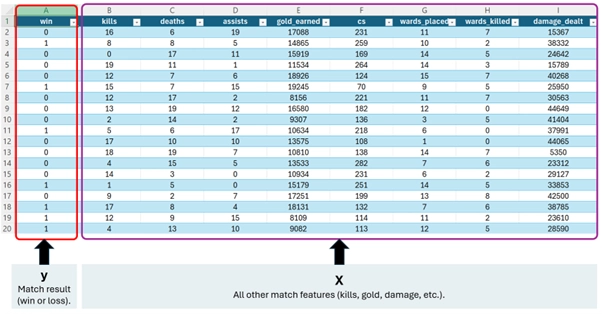
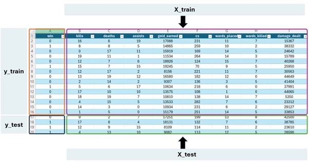
These screenshots are for illustration only, taken from a larger dataset with thousands of matches.
They show how we split the data into features (X) and target (y), then further divide it into training (80%) and testing (20%) sets.
3. Building the Logistic Regression Model
Now that our data is ready, it’s time to build a simple machine learning model: logistic regression.
Logistic regression is often used for binary classification—that means it helps us predict one of two possible outcomes. In our case:
1→ Win0→ Loss
We’ll use PyTorch to define the model. Don’t worry—it’s just a few lines of code!
What the model does:
Takes in match stats (kills, gold, damage, etc.).
Learns patterns from the training data.
Predicts the probability of winning the match.
How we build it:
Define the model class using PyTorch.
Use a sigmoid function to convert outputs to probabilities between 0 and 1.
Set the loss function to measure how far off our predictions are.
Choose an optimizer to help the model improve during training.
Here’s the basic code:
import torch.nn as nn
import torch.optim as optim

# 1. Define the model
class LogisticRegressionModel(nn.Module):
    def __init__(self, input_units):
        super(LogisticRegressionModel, self).__init__()
        self.linear = nn.Linear(input_units, 1)

    def forward(self, x):
        return torch.sigmoid(self.linear(x))  # Outputs probability (0 to 1)

# 2. Initialize the model
model = LogisticRegressionModel(input_units=X_train.shape[1])

# 3. Loss function: Binary Cross Entropy
criterion = nn.BCELoss()

# 4. Optimizer: Stochastic Gradient Descent
optimizer = optim.SGD(model.parameters(), lr=0.01)
You don’t need to memorize this code. Just understand the idea:
we’re building a simple model that learns to predict win/loss based on match stats. The full code is available at the end of this post if you want to explore it in detail.
4. Training the Logistic Regression Model
Now it’s time to teach our model how to predict. This process is called training—we show the model a lot of examples, let it make predictions, then correct it when it’s wrong.
Here’s what happens during training:
The model takes in training data.
It makes predictions (maybe wrong at first).
We calculate how wrong it was (this is called loss).
The model updates itself to do better next time.
We repeat this process many times. In our case, we’ll train the model for 1,000 rounds (epochs).
Steps in our training loop:
Set model to training mode
Zero the gradients (resetting previous updates)
Make predictions
Calculate the loss
Backpropagate (adjust internal weights, the actual learning process). See How Backpropagation Works in Neural Networks for a full explanation.
Update model parameters
Here’s what the code looks like:
epochs = 1000  # Number of training rounds

for epoch in range(epochs):
    model.train()  # Training mode
    optimizer.zero_grad()  # Reset gradients

    outputs = model(X_train).squeeze()  # Predictions
    loss = criterion(outputs, y_train)  # Calculate loss

    loss.backward()  # Backpropagation
    optimizer.step()  # Update model weights

    if epoch % 100 == 0:
        print(f"Epoch {epoch+1}, Loss: {loss.item():.4f}")
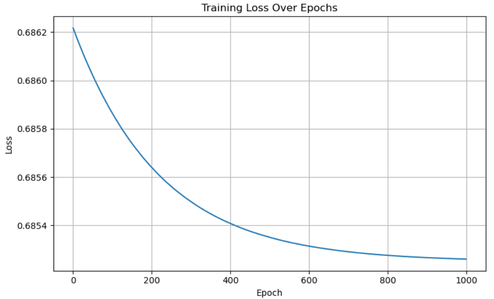
As training progresses, the loss value decreases, which means the model is getting better at predicting.
For example, you might see the loss go from 0.74 at the beginning to around 0.69 later—this tells us it’s learning!
5. Model Optimization and Evaluation
After training the model, it’s important to evaluate how well it performs—and see if we can make it even better.
One common technique to improve models is L2 Regularization (also called weight decay).
This helps prevent overfitting, which happens when a model memorizes the training data too closely and fails to perform well on new data.
Why do we need regularization?
Imagine a student who memorizes past exam answers but doesn’t understand the topic. He might do well on practice tests but fail on the real exam. Regularization helps the model generalize better to new data.
What we do here:
Apply L2 regularization by setting
weight_decay=0.01in the optimizer.Retrain the model using the same steps.
Evaluate the performance again on both training and testing sets.
Code snippet (just the key part):
# Optimizer with L2 regularization
optimizer = optim.SGD(model.parameters(), lr=0.01, weight_decay=0.01)
The rest of the training steps are the same as before.
After training, we check:
Accuracy on training data
Accuracy on test data
This tells us how well the model learned—and how well it performs on unseen matches.
If test accuracy improves (even a little), that’s a good sign the model is more reliable.
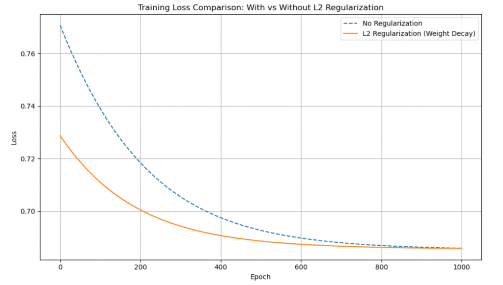
Although the loss curve may not show a dramatic difference, L2 regularization helps the model generalize better.
It slightly improves test accuracy and prevents overfitting—especially noticeable in more complex models or noisier datasets.
6. Visualizing LoL Match Prediction Results
Now that our model is trained and optimized, let’s visualize how well it performs. Numbers like accuracy are useful, but visuals make things much easier to understand.
We’ll look at three things:
1. Confusion Matrix
A confusion matrix helps us see:
How many wins and losses the model predicted correctly.
Where it made mistakes (e.g., predicting a win when it was actually a loss).
It splits predictions into 4 categories:
✅ True Positive (predicted win, actually win)
✅ True Negative (predicted loss, actually loss)
❌ False Positive (predicted win, actually loss)
❌ False Negative (predicted loss, actually win)
2. ROC Curve and AUC Score
ROC Curve shows how good the model is at separating wins from losses.
AUC (Area Under Curve) tells us how well the model performs overall (closer to 1 is better, 0.5 means guessing randomly).
3. Classification Report
This gives precision, recall, and F1-score for both win and loss predictions.
Here’s what the result might look like:
- The confusion matrix shows some incorrect predictions, but overall, the model is learning.
- The ROC curve helps confirm that the model is better than guessing.
- The classification report gives a detailed summary of how well each class (win/loss) is handled.
These visual tools are important in any classification task, not just for games. They help us understand the strengths and weaknesses of our model.
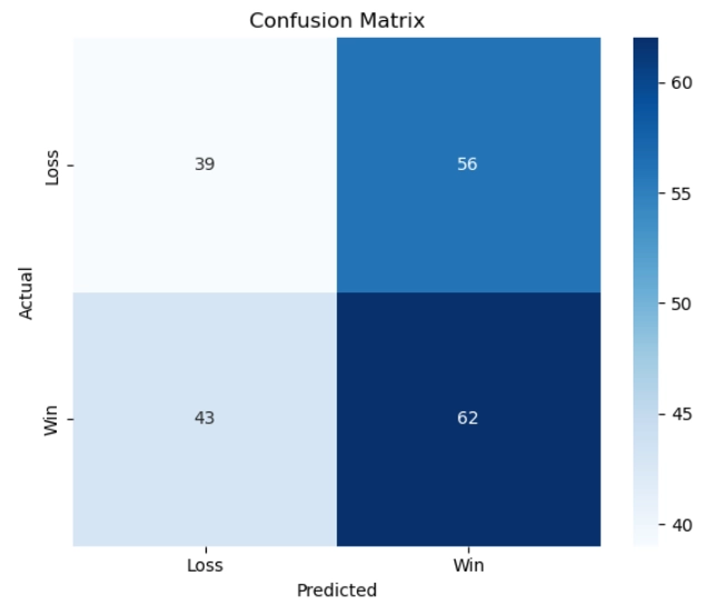
The matrix helps us see where the model got things right or wrong:
✅ 62 true wins, ✅ 39 true losses
❌ 43 false losses, ❌ 56 false wins
The model struggles with accuracy and balance, especially when predicting losses.
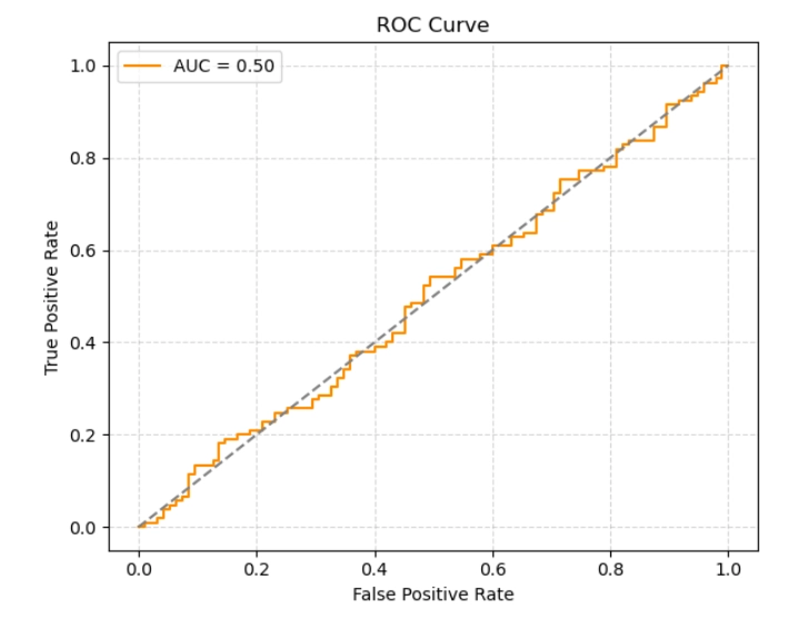
This ROC curve shows how well the model can distinguish between wins and losses. An AUC of 0.50 means it’s no better than flipping a coin—so there’s definitely room to improve!
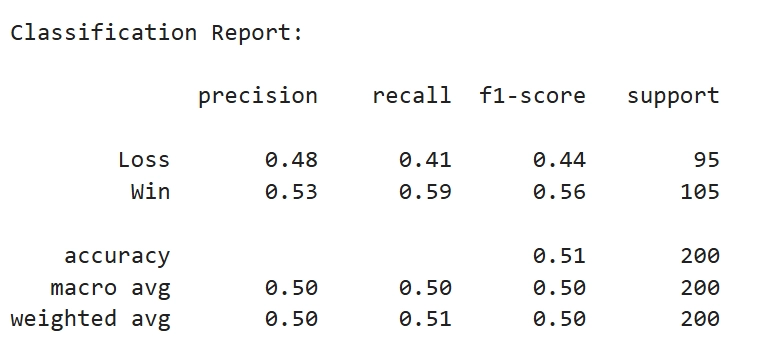
- Precision: How many predicted wins/losses were actually correct.
- Recall: How many actual wins/losses were captured correctly.
- F1-score: A balance between precision and recall.
Overall, the model reached 51% accuracy, which is slightly better than random but not strong enough for real use—good enough for learning, though!
7. Feature Importance
Now that we’ve trained and tested our model, let’s find out which features actually matter in predicting match outcomes.
In logistic regression, each feature has a weight (also called a coefficient). These weights tell us how much each feature influences the prediction.
What we’ll do:
Extract the weights from the model.
Match them with the original feature names.
Visualize them to see which stats (like kills or gold earned) had the most impact.
How to understand it:
A positive weight means the feature increases the chance of winning.
A negative weight means it decreases the chance.
A larger absolute value = more influence (whether positive or negative).
Visual Output (bar chart):
You’ll see a bar chart with features sorted by importance. This gives quick insight into what the model “thinks” matters most.
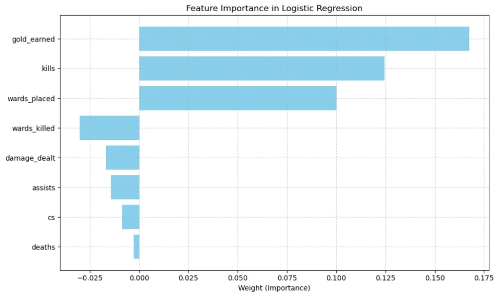
This chart shows which in-game statistics influenced the model’s predictions the most.
Features with higher weights (positive or negative) had more impact.
For example, gold earned and damage dealt had strong influence, while deaths had very little.
It’s a great way to understand what the model “learned” from the data.
8. Conclusion and Next Steps
We’ve now walked through the full journey of building a simple prediction model using logistic regression—and applied it to something fun and familiar: League of Legends match data.
What you’ve learned:
How to prepare and clean real-world data for machine learning.
How to build a logistic regression model using PyTorch.
How to train, evaluate, and optimize your model.
How to visualize results like confusion matrices and ROC curves.
How to interpret feature importance to understand what influences predictions.
Important Note:
This project was built for learning purposes. In real-world applications, more complex models like decision trees, ensemble methods, or deep learning would likely perform better on this kind of task.
However, what you’ve done here lays a solid foundation for understanding how machine learning works—and gives you the tools to go even further!
Full Project Code
You can find the full code for this project, including all steps and visualizations, on my GitHub:
What’s next?
Try using other models like Random Forest or Neural Networks.
Add more features or clean the data in different ways.
Test on other datasets—sports, games, or even your own!
If you want to dive deeper into the math behind logistic regression, check out this excellent explanation in the Scikit-learn documentation.
Machine learning is all about experimenting, learning, and improving. Keep exploring, and have fun doing it!

